A highly targeted phishing campaign has been hitting hotel guests across Luxembourg. Originally flagged by the Computer Incident Response Center Luxembourg (CIRCL), this campaign stands out not because of advanced malware, but because of its impeccable contextual credibility . Threat actors aren't guessing targets; they are hitting actual hotel guests on WhatsApp with exact, legitimate booking details to steal credit card data. As part of a technical review into the infrastructure, we analyzed a recent Indicator of Compromise (IoC) linked to this campaign: [https://stay-hotel607923.com](https://stay-hotel607923.com) . Here is the deep dive into how this attack works, the infrastructure behind it, and how to track it. The Attack Workflow: Smishing with Context Most phishing campaigns rely on volume, hoping a small fraction of a massive email list bites. This campaign relies on precision. The Data Exposure: CIRCL assesses that the campaign's source data may originate from servi...
With Malware exploding in numbers, I decided to learn and apply Data Science to Malware.
So first I need a number of Malware samples, which I obtained from https://github.com/fabrimagic72/malware-samples
Now the following techniques can work on any set of Malware, maybe if your a business/organization who is being targeted or you’ve been following a certain group of Malware authors and you want to see how the Malware is connected, if they use the same resources, hosts, code, etc then that would yield some interesting data and start to paint a picture.
Unfortunately, I don’t have access to those sets of Malware but that doesn’t say we can’t apply the techniques to Malware collected from honeypots.
Ransomeware samples
From the Malware samples, the Ransomware folder looks to have a number of samples we could apply the techniques on.
Step one: unzip all the Malware within that dir:
find . -name “*.zip” | while read filename; do 7z x $filename -pinfected -aou; done;
Step two: start building the script
Now I won’t post the whole script on here, I’ll add a link at the bottom it once I put it up on Github.
Step two: start building the script
Now I won’t post the whole script on here, I’ll add a link at the bottom it once I put it up on Github.
So let’s take a look at the interesting stuff:
for root,dirs,files in os.walk(args.target_path):
for path in files:
#try opening the file with pe to see if it’s really a pe file
try:
pe = pefile.PE(os.path.join(root,path))
except pefile.PEFormatError:
continue
fullpath = os.path.join(root,path)
#extract printable strings from the target sample
strings = os.popen(“strings ‘{0}’”.format(fullpath)).read()
#use the search_doc function in the included reg mod, to find hostnames
hostnames = find_hostname(strings)
if len(hostnames):
#add the nodes and edges for the bipartite network
network.add_node(path,label=path[:32],color=’black’,penwidth=5,bipartite=0)
for hostname in hostnames:
network.add_node(hostname,label=hostname,color=’blue’,penwidth=10,bipartite=1)
network.add_edge(hostname,path,penwidth=2)
#NOTE WE HAVE EXTRACTED ALL MALWARE INTO ONE FOLDER
if hostnames:
print “extracted hostnames from:”,path
pprint.pprint(hostnames)
What this does, is looks through each file in the given directory, check if it has a PE header if so we run the program “strings” on it, then get the list of strings from the file and run it through a function called “find_hostname” (which I’ve not posted here, but it goes through a regex process to strip the input and run the list through a list of domain suffixes to say if it string matches a list within domain suffixes, then it is accepted as a domain)
Then we create our network.
If we have a positive list of hostname, we’ll create a node for that malware.
network.add_node(path,label=path[:32],color=’black’,penwidth=5,bipartite=0)
Now we’ll start to create nodes and edges for each hostname we find that is connected to that malware.
network.add_node(hostname,label=hostname,color=’blue’,penwidth=10,bipartite=1)
network.add_edge(hostname,path,penwidth=2)
And then print the hostname to the screen.
And the results are, to me anyway, interesting. We can see the following
hostnames:
extracted hostnames from smb-b4tq2hti.bin
[‘mnses7xf743znk7.onion’,
‘r5x6sdidz4q7f6q.onion’,
‘sw7xmbs2ivmt5og.onion’,
Note — I have removed some characters from the hostname, safety first :)
Now let’s save everything to a “.dot” file so that we can convert the network into a visual graph.
#write the dot file to disk
write_dot(network,args.output_file)
malware = set(n for n, d in network.nodes(data=True) if d[‘bipartite’]==0)
hostname = set(network)-malware
#use networkX’s bipartite network projection function to produce the malware and hostname projections
malware_network = bipartite.projected_graph(network, malware)
hostname_network = bipartite.projected_graph(network, hostname)
#write the projected networks to disk as specified by the user
write_dot(malware_network, args.malware_projection)
write_dot(hostname_network,args.hostname_projection)
So we will have 3 files, the first being the whole network, the second to show the connection between the Malware, and the third to show the connections between the hostnames.
python ransomewareMalwareNetwork.py /home/osboxes/myAnalysis/malware-samples/Ransomware/extracted ./orginal.dot ./malwareProjection.dot ./hostname_projection.dot
We then use fdp (one of many choices but it is suited for a small network) to convert the “.dot” files into images:
fdp orginal.dot -T png -o orignal_ransomeware_image.png
And now let’s view the results:
Original network, showing the connection between the Malware and hostnames:
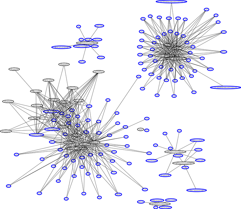
The blue circle represents hostnames and the black circle represents the Malware. Now, granted it’s quite hard to actually see the connection via Medium but this was something I was hoping to see.
The cluster on the left is from the “Wannacry” folder and we would expect to see those files and hostnames linked.
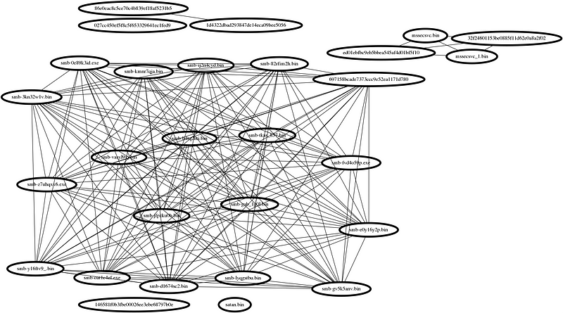
Next, let’s view just the Malware connections:
And the hostname projection:
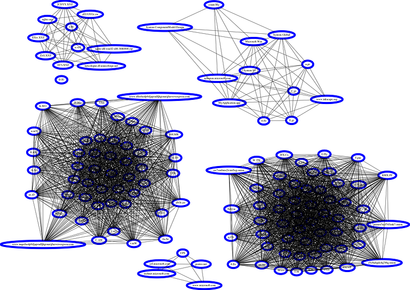
Now, visually the hostname doesn’t tell us much, so that’s going to take me some time to adjust the network for the hostname to get it to be more visually pleasing and useful.
I won’t do a review of my findings as this is just to apply what I learn to some real-world Malware. And I’m quite happy with the findings and itching to see how else we can use the data we learn from Malware via Malware analysis and add it to these methods.
Now, I did try to build a graph based on image relationship for the ransomware malware, which is done by extracting the images from the malware but the results were far less “exciting” but that could be because the malware doesn’t use images or it is obfuscated.
Either way, we can use the same methods on different samples to see what they yeild.
Everything I learned and applied in the above is from the book “Malware Data Science”. I highly recommend it.
Comments
Post a Comment