A highly targeted phishing campaign has been hitting hotel guests across Luxembourg. Originally flagged by the Computer Incident Response Center Luxembourg (CIRCL), this campaign stands out not because of advanced malware, but because of its impeccable contextual credibility . Threat actors aren't guessing targets; they are hitting actual hotel guests on WhatsApp with exact, legitimate booking details to steal credit card data. As part of a technical review into the infrastructure, we analyzed a recent Indicator of Compromise (IoC) linked to this campaign: [https://stay-hotel607923.com](https://stay-hotel607923.com) . Here is the deep dive into how this attack works, the infrastructure behind it, and how to track it. The Attack Workflow: Smishing with Context Most phishing campaigns rely on volume, hoping a small fraction of a massive email list bites. This campaign relies on precision. The Data Exposure: CIRCL assesses that the campaign's source data may originate from servi...
Shared code analysis
In the last section, I wrote about building networks and producing a visual graph that shows the connections between Malware.
In this section, I will go through the script where we create a system that will show the links between Malware based on shared code analysis.
Terminology
Before we start to build the system, we first need to understand the following:
1. Jaccard index
2. Minhashes
Jaccard index
The Jaccard index is quite simple, it is worked out by diving the total of shared attributes (between malware) and the total attributes.
For example:
Jaccard index = 0.5 when shared attributes (5) / total attributes (10).
Now, this is useful for small data sets, but when we want to compare large data sets then we turn to “minhashes”.
Minhashes
Now Minhashes isn’t so simple.
A minhash is a technique used to estimate the similarity of two sets.
Our minhash is a malware sample’s feature (in our below system the features will be the results from “strings”) and is hashed with k hash function and we take the minimum value of the hashes from all the features that were hashed, this is to reduce the set of malware features to a fixed size array of k integers, which we call minhashes.
With the minhashes, we can calculate our “Jaccard index” between two samples. We just check how many minhashes match and divide that by k.
Hopefully, once I show the code and talk through it, it will become more apparent what a minhash is. But one of the main reasons for using minhash is because it’s faster than using the Jaccard method when we have a large dataset.
A good video for a more in-depth look into the above: https://www.youtube.com/watch?v=aTwRpqUnQX8
Building the system
The malware will be analyzed based on their strings features (In the future we will add different features to this system, but let's go one step at a time).
import sys
import argparse
import os
import murmur
import shelve
import numpy as np
from similarity_graph import *
NUM_MINHASHES = 256
SKETCH_RATIO = 8
The “similarity_graph” is the code from part 1, as we will reuse the same functions for checking if the file is a PE file and getting the strings.
The minhash and sketch ratio (sketching is used with minhash) is set based on the values from the book Malware data science.
Now like before, I won’t post all the code I used to build the system as I want to talk about the main features used to build it, but you can find it on my Github — https://github.com/cchaq/MalwareDataScience
First up, the minhash function:
def minhash(features):
minhashes = []
sketches = []
for num_minhash in range(NUM_MINHASHES):
minhashes.append(
min([murmur.string_hash(‘feature’, num_minhash) for feature in features])
)
for i in xrange(0,NUM_MINHASHES,SKETCH_RATIO):
sketch = murmur.string_hash(‘minhashes[i:i+SKETCH_RATIO]’)
sketches.append(sketch)
return np.array(minhashes),sketches
We have a “features” parameter which in this instance will be from our “strings” result (which we’ll go through later).
We’ll create our minhashes and sketches array because we’ll want to add these to our database.
The for loop will iterate through NUM_MINHASHES, so 256 times, and append our minhashes array with a hashed feature.
For hashing the murmur library is used, after reading about it, it is a good hashing library to use because it’s fast (other reasons as well but speed is the main focus here). A quick run-through of the murmur.string_hash function reveals how our “hashed” features will be stored:
>>> import murmur
>>> murmur.string_hash(‘feature’,1)
3486256588
Once we’ve gone through the number of hashes (256), we’ll take the minimum hash value and add it to our array.
Next, we iterate through the minhashes and use them to create our sketches. A sketch is a hash of multiple minhashes, in this case, we set the ratio to 8, which we use for database indexing of our malware samples. This will speed up the retrieval process of malware that are likely to be similar to one another. We have to remember that this database could grow considerably in size, which is why there is indexing.
Building the database
Now, let’s build the database.
def store_sample(path):
db = get_database()
features = getstrings(path)
minhashes, sketches = minhash(features)
for sketch in sketches:
sketch = str(sketch)
if not sketch in db:
db[sketch] = set([path])
else:
obj = db[sketch]
obj.add(path)
db[sketch] = obj
db[path] = {‘minhashes’:minhashes,’comments’:[]}
db.sync()
print “Extracted {0} features from {1}…”.format(len(features),path)
Remember, the “getstrings” function is from the “similarity_graph” script we created in the previous section. This will build our list of features (the result from “strings”) and that is passed into the minhash function which we covered above.
We iterate over our sketches and add if it does not exist in the database, we create the record and use the sample malware file path as the ID.
Now, if the sketch does exist then we add the sample malware file path to the sketch’s set of associated sample paths.
After adding the sketches to the database with the path as the ID, we set our minhashes to the path.
Searching for similar malware samples
The code:
def search_sample(path):
db = get_database()
features = getstrings(path)
minhashes, sketches = minhash(features)
neighbours = []
for sketch in sketches:
sketch = str(sketch)
if not sketch in db:
continue
for neighbour_path in db[sketch]:
neighbour_minhashes = db[neighbour_path][‘minhashes’]
similarity = (neighbour_minhashes == minhashes).sum() / float(NUM_MINHASHES)
neighbours.append((neighbour_path, similarity))
neighbours = list(set(neighbours))
neighbours.sort(key=lambda entry:entry[1],reverse=True)
print “”
print “Sample name”.ljust(64),”Shared code estimate”
for neighbour, similarity in neighbours:
short_neighbour = neighbour.split(“/”)[-1]
comments = db[neighbour][‘comments’]
print str(“[*] “+short_neighbour).ljust(64),similarity
for comment in comments:
print “\t[comment]”,comment
With this function, we can pass compare malware samples without having to load them to our database, although having to go through the process of getting the hashes for malware samples we passed through again is a redundant process, something to work on in the future.
We iterate over the malware sample sketches and for each sketch, we will look up the stored malware samples.
After that, we’ll work out the Jaccard index:
similarity = (neighbour_minhashes == minhashes).sum() / float(NUM_MINHASHES)
The results
Ok, so I mentioned the main functions of the system except one which is to search for the samples, but I will do a separate write up for that as it’s could make this write up a bit long-winded.
Now you will also see some seem arguments passed in when I run the script and if you want to see how they are implemented then please check out the full code on my GitHub page — https://github.com/cchaq/MalwareDataScience
First, we will load our malware samples features into the database:
python minhash_relation.py -l /home/osboxes/myAnalysis/malware-samples/Ransomware/extracted
Extracted 8388 features from /home/osboxes/myAnalysis/malware-samples/Ransomware/extracted/smb-d1674sc2.bin…
Extracted 7538 features from /home/osboxes/myAnalysis/malware-samples/Ransomware/extracted/smb-fvd4o59p.exe…
Extracted 1793 features from /home/osboxes/myAnalysis/malware-samples/Ransomware/extracted/smb-jfpzku0b.bin…
Extracted 632 features from /home/osboxes/myAnalysis/malware-samples/Ransomware/extracted/1d4322dbad293847de14eca09bee5056eaede7ce178490e101642bf1f5875e37…
Extracted 9227 features from /home/osboxes/myAnalysis/malware-samples/Ransomware/extracted/smb-ij2n4cyd.bin…
Extracted 6032 features from /home/osboxes/myAnalysis/malware-samples/Ransomware/extracted/smb-gv5k5anv.bin…
Extracted 3602 features from /home/osboxes/myAnalysis/malware-samples/Ransomware/extracted/smb-e0y16y2p.bin…
Extracted 305 features from /home/osboxes/myAnalysis/malware-samples/Ransomware/extracted/smb-ojjfqxul.bin…
Extracted 44463 features from /home/osboxes/myAnalysis/malware-samples/Ransomware/extracted/32f24601153be0885f11d62e0a8a2f0280a2034fc981d8184180c5d3b1b9e8cf.bin…
If we open our database file via the Python command line and print it’s data, this is what we see:
>>> import shelve
>>> db = shelve.open(“samples.db”)
>>> dbkeys = list(db.keys())
>>> for key in dbbeys:
… print (key,db[key])
(‘/home/osboxes/myAnalysis/malware-samples/Ransomware/extracted/146581f0b3fbe00026ee3ebe68797b0e57f39d1d8aecc99fdc3290e9cfadc4fc.bin’, {‘minhashes’: array([231
5179632, 3486256588, 1845446934, 574354670, 3634204494,
3868613078, 3316310169, 730525171, 545429338, 4253172697,
2757105328, 408003201, 217562801, 1661354022, 2763938731,
1059248515, 2107807121, 1885863305, 3307288677, 1587378795,
27164293, 3793397666, 400853354, 2192977244, 2594248640,
2141616303, 3335467927, 1221082220, 203908147, 2346593753,
(‘2843819777’, set([‘/home/osboxes/myAnalysis/malware-samples/Ransomware/extracted/32f24601153be0885f11d62e0a8a2f0280a2034fc981d8184180c5d3b1b9e8cf.bin’, ‘/hom
e/osboxes/myAnalysis/malware-samples/Ransomware/extracted/smb-ij2n4cyd.bin’, ‘/home/osboxes/myAnalysis/malware-samples/Ransomware/extracted/smb-fvd4o59p.exe’,
‘/home/osboxes/myAnalysis/malware-samples/Ransomware/extracted/smb-3kn32w1v.bin’, ‘/home/osboxes/myAnalysis/malware-samples/Ransomware/extracted/smb-0e89k3id.e
xe’, ‘/home/osboxes/myAnalysis/malware-samples/Ransomware/extracted/satan.bin’, ‘/home/osboxes/myAnalysis/malware-samples/Ransomware/extracted/smb-d1674sc2.bin
‘, ‘/home/osboxes/myAnalysis/malware-samples/Ransomware/extracted/697158bcade7373ccc9e52ea1171d780988fc845d2b696898654e18954578920’, ‘/home/osboxes/myAnalysis/
malware-samples/Ransomware/extracted/smb-gv5k5anv.bin’, ‘/home/osboxes/myAnalysis/malware-samples/Ransomware/extracted/smb-y16ftv9_.bin’, ‘/home/osboxes/myAnal
ysis/malware-samples/Ransomware/extracted/smb-kmnr7qja.bin’, ‘/home/osboxes/myAnalysis/malware-samples/Ransomware/extracted/smb-e0y16y2p.bin’, ‘/home/osboxes/m
yAnalysis/malware-samples/Ransomware/extracted/smb-b4tq2hti.bin’, ‘/home/osboxes/myAnalysis/malware-samples/Ransomware/extracted/smb-gab_1g0l.bin’, ‘/home/osbo
xes/myAnalysis/malware-samples/Ransomware/extracted/smb-tkas_857.bin’, ‘/home/osboxes/myAnalysis/malware-samples/Ransomware/extracted/mssecsvc.bin’, ‘/home/osb
oxes/myAnalysis/malware-samples/Ransomware/extracted/smb-82rfim2h.bin’, ‘/home/osboxes/myAnalysis/malware-samples/Ransomware/extracted/smb-jfpzku0b.bin’, ‘/hom
e/osboxes/myAnalysis/malware-samples/Ransomware/extracted/smb-7rwkaozq.bin’, ‘/home/osboxes/myAnalysis/malware-samples/Ransomware/extracted/027cc450ef5f8c5f653
329641ec1fed91f694e0d229928963b30f6b0d7d3a745’, ‘/home/osboxes/myAnalysis/malware-samples/Ransomware/extracted/smb-z7uhqxx6.exe’, ‘/home/osboxes/myAnalysis/mal
ware-samples/Ransomware/extracted/ed01ebfbc9eb5bbea545af4d01bf5f1071661840480439c6e5babe8e080e41aa.bin/ed01ebfbc9eb5bbea545af4d01bf5f1071661840480439c6e5babe8e
080e41aa.bin (1)’, ‘/home/osboxes/myAnalysis/malware-samples/Ransomware/extracted/smb-lyqgstbu.bin’, ‘/home/osboxes/myAnalysis/malware-samples/Ransomware/extra
cted/smb-oat1c4ef.exe’, ‘/home/osboxes/myAnalysis/malware-samples/Ransomware/extracted/86e0eac8c5ce70c4b839ef18af5231b5f92e292b81e440193cdbdc7ed108049f.bin’, ‘
/home/osboxes/myAnalysis/malware-samples/Ransomware/extracted/1d4322dbad293847de14eca09bee5056eaede7ce178490e101642bf1f5875e37’, ‘/home/osboxes/myAnalysis/malw
are-samples/Ransomware/extracted/smb-ojjfqxul.bin’, ‘/home/osboxes/myAnalysis/malware-samples/Ransomware/extracted/mssecsvc_1.bin’, ‘/home/osboxes/myAnalysis/m
alware-samples/Ransomware/extracted/146581f0b3fbe00026ee3ebe68797b0e57f39d1d8aecc99fdc3290e9cfadc4fc.bin’, ‘/home/osboxes/myAnalysis/malware-samples/Ransomware
/extracted/smb-vasyl9yj.bin’]))
Now that we have loaded the Malware samples hashes, let’s test the results of the shared code estimate:
python minhash_relation.py -s ~/myAnalysis/malware-samples/Ransomware/extracted/smb-82rfim2h.bin
Oh, I forgot to mention that the samples I load are the same as my previous post.
And the result:
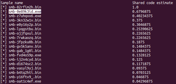
Shared code estimate for smb-82rfim2h.bin
We can see that it shares a code estimate of 1 with itself (no surprise there) and the next Malware sample it has a close relationship with is “smb-0e89k3id.exe”
After that, the numbers start to drop but we can still see that the Ransomeware sample does share some common “features” (that being the result from our “strings”.
Now, what would be interesting to see is if we start to grow our feature list, what kind of results would it yield and by building a database, everything we add new Malware we can see if it shares code with previously loaded Malware or if it’s from a new group.
Comments
Post a Comment